
|
"The woods, lovely, dark and deep,
are to be seen on foot."
|
Contents
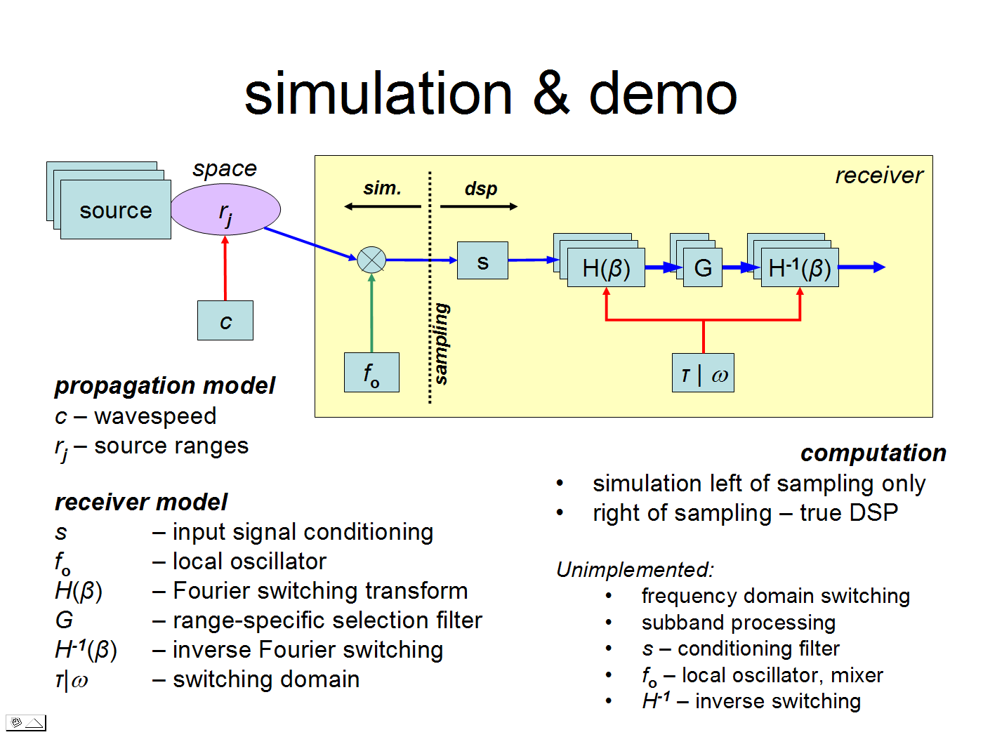
What is simulated
The applet above simulates sources and applies
continuously varied Fourier spectrum analysis
by varying
the sampling intervals.
As can be seen from the applet,
this results in scaling of the individual source spectra
in proportion to the source distances,
even though
the source distances are not input to
either the sampling or the FFT.
There are three scenarios configured in this applet instance
to demonstrate this effect.
- fibre:
Sources and propagation in an optical fibre
of core refractive index 1.47.
A large range of values is applied to
the Fourier analysis variation, or switching, rate
to demonstrate the scalability of the effect.
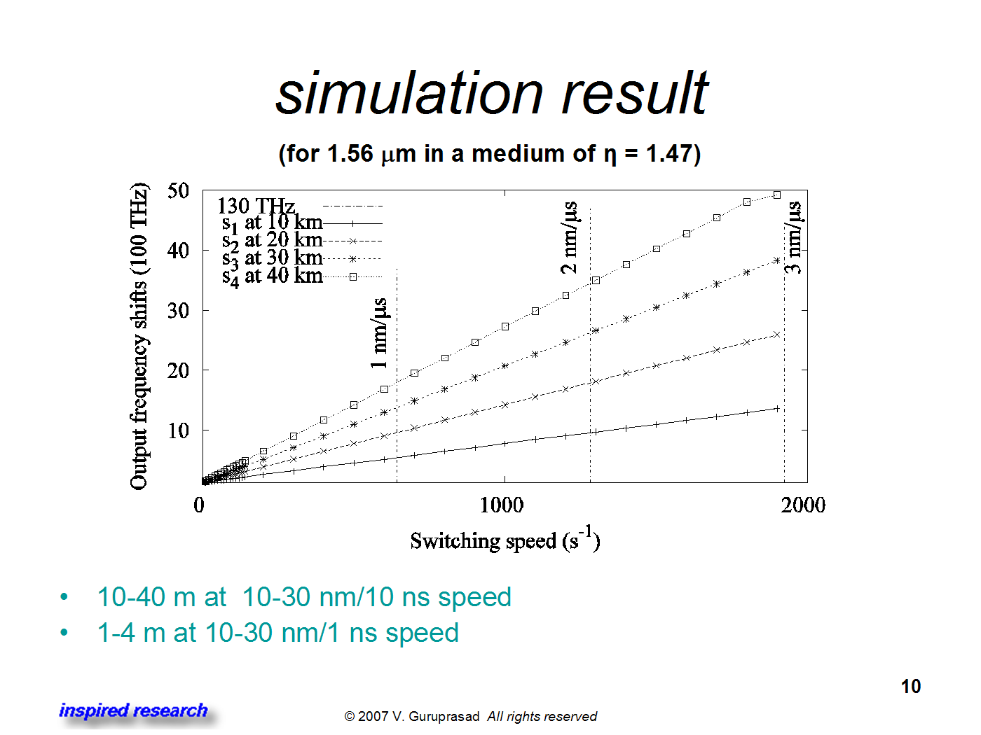
- fibre-plot:
The same set but with the Fourier switching rates programmed
over two narrow ranges
to demonstrate the linearity
-- see result graph.
- cosmic:
Sources and propagation over astronomical distances,
in this case, on the lunar range.
(This is really a limitation of the 32-bit Java virtual machine
and its trigonometric library.)
The scenario is selected by a choice button
in the middle left region of the applet,
and is executed by selecting successive indices of the scenario.
For example, the first scenario requires picking
the choices
--fibre--
fibre1
fibre2
...
--end-fibre--
in succession.
Note that --fibre-- and --cosmic-- merely set up
the environment parameters.
The respective sources are only loaded in
fibre1 and cosmic1, respectively,
and are cleared in the end markers.
There is online help explaining the use of the control panel
at the bottom right of the applet - the choice button right of
the applet title brings up the help text in the rectangular text area.
Some features shown are yet to be implemented, viz
reverse switching (H*),
subband filtering,
and
frequency domain Fourier switching.
A key feature is the simulation of source linespreds,
controlled by the checkboxes labelled ∼ and ≡
bottom left of the applet.
The first causes each source, in effect, to be producing its output
at spectral shifts of δ
-- notice that this linespread shift is at the input to the sampling,
and is NOT proportional to the source distances.
The second causes the arriving phase to be calculated as the mean over
all possible shifts over the range [0, δ)
-- which are again NOT proportional to source distances.
The results turn out to be the same, except that
the second choice takes up more compute time and memory space.
What the simulation does NOT prove
-
Adequate linespreads from terrestrial and artificial sources.
Adequate linespreads can be incidentally taken for granted for astronomical sources
because they are almost always
at high enough temperature to emit radiation,
and
the required linespread to produce the observed redshifts is extremely small,
of the order of
β = -10-18 s-1.
-
Sufficiency of variable sampling to extract chirps.
The extraction is
a direct mathematical result of the wave equation
and a changing receiver,
as explained in
the published patent application and
the IEEE conference papers of 2005.
Simulation was necessary only to verify that
the result is tenable.
The test of any new physics has to be empirical.
-
Necessity of variable sampling for the phase acceleration effect.
The same chirps and distance-dependent shifts are incidentally obtained
even on commenting out the sampling rate variation
in the sampling code
so long as
the linespreading simulation is retained,
as
the linespreading alone suffices to yield chirps.
We don't get the same behaviour
in traditional spectrometers or DFT
because
the summing process in digital or analogue spectrometry
accentuates the spectral lines,
suppressing the linespreads.
In a real or DSP spectrometer dealing
with real waves and linespreads,
variable sampling (or its equivalent) remains necessary
to suppress the summation.
